


 Download code from GitHub
Chapter 1
Foundations of Quantum Computing
The beginning is always today.
— Mary Shelley
You may have heard that the mathematics needed to understand quantum computing is arcane, mysterious and difficult…but we utterly disagree! In fact, in this chapter, we will introduce all the concepts that you will need in order to follow the quantum algorithms that we will be studying in the rest of the book. Actually, you may be surprised to see that we will only rely on some linear algebra and a bit of (extremely simple) trigonometry.
We shall start by giving a quick overview of what quantum computing is, what the current state of the art is, and what the main applications are expected to be. After that, we will introduce the model of quantum circuits. There are several computational models for quantum computing, but this is the most popular one and, moreover, it's the one that we will be using throughout most of the book. Then, we will describe in detail what qubits are, how we can operate on them by using quantum gates, and how we can retrieve results by performing measurements. We will start with the simplest possible case — just a humble qubit! Then, we will steadily build upon that until we learn how to work with as many qubits as we want.
This chapter will cover the following topics:
Quantum computing: the big picture
The basics of the quantum circuit model
Working with one qubit and the Bloch sphere
Working with two qubits and entanglement
Working with multiple qubits and universality
After reading this chapter, you will have acquired a solid understanding of the fundamentals of quantum computing and you will be more than ready to learn how practical quantum algorithms are developed.
1.1 Quantum computing: the big picture
In October 2019, an announcement made by a team of researchers from Google took the scientific world by storm. For the first time ever, a practical demonstration of quantum computational advantage had been shown. The results, published in the prestigious Nature journal [9], reported that a quantum computer had solved, in just a few minutes, a problem that would have taken the most powerful classical supercomputer in the world thousands of years.
Although the task solved by the quantum computer has no direct practical applications and it was later claimed that the computing time with classical resources had been overestimated (see [75] and, also, [73]), this feat remains a milestone in the history of computing and has fueled interest in quantum computing all over the world. So, what can these mysterious quantum computers do? How do they work in order to achieve these mind-blowing speed-ups?
We could define quantum computing as the study of the application of properties of quantum systems (such as superposition, entanglement, and interference) to accelerate some computational tasks. These properties do not manifest in our macroscopic world and, although they are present at the fundamental level in our computing devices, they are not explicitly used in the traditional computing models that we employ to build our microprocessors and to design our algorithms. For this reason, quantum computers behave in a radically different way to classical computers, making it possible to solve some tasks much more efficiently than with traditional computing devices.
The most famous problem for which quantum algorithms offer a huge advantage over classical methods is finding prime factors of big integers. The best known classical algorithm for this task requires an amount of time that grows almost exponentially with the length of the number (see Appendix C, Computational Complexity, for all the concepts referred to computational complexity, including exponential growth). Thus, factoring numbers that are several thousand bits long becomes infeasible with classical computers, and this inefficiency is the basis for some widely used cryptographic protocols, such as RSA, proposed by Rivest, Shamir, and Adleman [80].
Nevertheless, more than twenty years ago, the mathematician Peter Shor proved in a celebrated paper [87] that a quantum computer could factor numbers taking an amount of time that no longer grows exponentially with the size of the input, but only polynomially. Other examples in which quantum algorithms outperform classical ones include finding elements satisfying a given condition from an unsorted list (with Grover's algorithm [48]) or sampling from the solutions of systems of linear equations (using the famous HHL algorithm [49]).
Wonderful as the properties of these quantum algorithms are, they require quantum computers that are fault tolerant and more powerful than those available today. This is why, in the last few years, many researchers have focused on studying quantum algorithms that try to obtain some advantage with the noisy intermediate-scale quantum computers, also known as NISQ devices, that are at our disposal now. The NISQ name was coined by John Preskill in a greatly enjoyable article [78] and has been widely adopted to describe the evolutionary stage in which quantum hardware currently is.
Machine learning and optimization are two of the fields that are being actively explored in this NISQ era. In these areas, many interesting algorithms have been proposed in recent years; some examples are the Quantum Approximate Optimization Algorithm (QAOA), the Variational Quantum Eigensolver (VQE), or different quantum flavors of machine learning models, including Quantum Support Vector Machines (QSVMs) and Quantum Neural Networks (QNNs).
Since these algorithms are fairly new, we still lack a complete understanding of their full capabilities. However, some partial theoretical results show some evidence that these approaches can offer some advantages over what is possible with classical computers, for instance, by giving us better approximations to the solutions of hard combinatorial optimization problems or by showing better performance when learning from particular datasets.
Exploring the real possibilities of these NISQ computers and the algorithms designed to take advantage of them will be crucial in the short and medium term, and it may very likely pave the way for the first practical applications of quantum computing to real-world problems.
We believe that you can be part of the exciting task of making quantum computing applications a reality and we would like to help you on that journey. But, for that, we need to start by setting in place the tools that we will be using throughout the book.
If you are already familiar with the quantum circuit model, you can skip the rest of this chapter. However, we recommend that you at least skim through the following sections so that you can get familiar with the conventions and choices of notation that we will use in this book.
1.2 The basics of the quantum circuit model
We have mentioned that quantum computing relies on quantum phenomena such as superposition, entanglement, and interference to perform computations. But what does this really mean? To make this explicit, we need to define a particular computational model that allow us to describe mathematically how to take advantage of all these properties.
There are many such models, including quantum Turing machines, measurement-based quantum computing (also known as one-way quantum computing), or adiabatic quantum computing, and all of them are equivalent in power. However, the most popular one — and the one that we will be using for the most part in the book — is the quantum circuit model.
To learn more…
In addition to the quantum circuit model, sometimes we will also use the adiabatic model. All the necessary concepts will be introduced in Chapter 4, Quantum Adiabatic Computing and Quantum Annealing.
Every computation has three elements: data, operations, and output. In the quantum circuit model, these correspond to some concepts that you may have already heard about: qubits, quantum gates, and measurements. Through the remainder of this chapter, we will briefly review all of them, highlighting some special details that will be of particular importance when talking about quantum machine learning and quantum optimization algorithms; at the same time, we will show the notation that will be used throughout the book. But before committing to that, let us have a quick overview of what a quantum circuit is.
Let's have a look at Figure 1.1. It shows a simple quantum circuit. The three horizontal lines that you see are sometimes called wires, and they represent the qubits that we are working with. Thus, in this case, we have three qubits. The circuit is meant to be read from left to right, and it represents all the different operations that are performed on the qubits. It is customary to assume that, at the very beginning, all the qubits are in state  . You do not need to worry yet about what means, but please notice how we have indicated that this is indeed the initial state of all the wires by writing to the left of each of them.

In that circuit, we start by applying an operation called a  gate on the top qubit; we will explain in the next section what all of these operations do, but note that we represent them with little boxes with the name of the operation inside. After that initial gate, we apply individual gates
  ,
,  , and
, and  on the top, middle, and bottom qubits and, then, a two-qubit gate on the top and middle qubits followed by a three-qubit gate, which acts on all the qubits at the same time. Finally, we measure the top and bottom qubits (we will get to measurements in the next section, don't worry), and we represent this in the circuit using the gauge symbol. Notice that, after these measurements, the wires are represented with double lines, to indicate that we have obtained a result — technically, we say that the state of the qubit has collapsed to a classical value. This means that, from this point on, we do not have quantum data anymore, only classical bits. This collapse may seem a little bit mysterious (it is!), but don't worry. In the next section, we will explain in detail the process by which quantum information (qubits) is transformed into classical data (bits).
As you may have noticed, quantum circuits are somewhat similar to digital ones, in which we have wires representing bits and different logical gates such as AND, OR, and NOT acting on them. However, our qubits, quantum gates, and measurements obey the rules of quantum mechanics and show some properties that are not found in classical circuits. The rest of this chapter is devoted to explaining all of this in detail, starting with the simplest of cases, that of a single qubit, but growing all the way up to fully-fledged quantum circuits that can use as many qubits and gates as desired.
Ready? Let's start, then!
1.3 Working with one qubit and the Bloch sphere
One of the advantages of using a computational model is that you can forget about the particularities of the physical implementation of your computer and focus instead on the properties of the elements on which you store information and the operations you can perform on them. For instance, we could define a qubit as a (physical) quantum system that is capable of being in two different states. In practice, it could be a photon with two possible polarizations, a particle with two possible values for its spin, or a superconducting circuit, whose current can be flowing in one of two directions. When using the quantum circuit model, we can forget about those implementation details and just define a qubit…as a mathematical vector!
1.3.1 What is a qubit?
In fact, a qubit (short for quantum bit, sometimes also written as qbit, Qbit or even q-bit) is the minimal information unit in quantum computing. In the same way that a bit (short for binary digit) can be in state  or in state
  , a qubit can be in state or in state
  . Here, we are using the so-called Dirac notation, where these funny-looking symbols surrounding and are called kets and are used to indicate that we are dealing with vectors instead of regular numbers. In fact, and are not the only possibilities for the state of a qubit and, in general, it could be in a superposition of the form

where  and
and  are complex numbers, called amplitudes, such that
  . The quantity
  is called the norm or length of the state and, when it is equal to , we say that the state is normalized.
To learn more…
If you need a refresher on complex numbers or vector spaces, please check Appendix A, Complex Numbers, and Appendix B, Basic Linear Algebra.
All these possible values for the state of a single qubit are vectors that live in a complex vector space of dimension 2 (in fact, they live in what is called a Hilbert space, but since we will be working only with finite dimensions, there is no real difference). Thus we shall fix the vectors and as elements of a special basis, which we will refer to as the computational basis. We will represent these vectors, constituents of the computational basis, as the column vectors

and hence

If we are given a qubit and we want to determine or, rather, estimate its state, all we can do is perform a measurement and get one of two possible results: 0 or 1. We have nonetheless seen how a qubit can be in infinitely many states, so how does the state of a qubit determine the outcome of a measurement? As you likely already know, in quantum physics, these measurements are not deterministic, but probabilistic. In particular, given any qubit  , the probability of getting upon a measurement is
  , while that of getting is
  . Naturally, these two probabilities must add up to 1, hence the need for the normalization condition .
If upon measuring a qubit we get, let's say, , we then know that, after the measurement, the state of the qubit is , and we say that the qubit has collapsed into that state. If we obtain , the state collapses to . Since we are obtaining results that correspond to and , we say that we are measuring in the computational basis.
Exercise 1.1
What is the probability of measuring 0 if the state of a qubit is  ? And the probability of measuring 1? What if the state of the qubit is
  ? And if it is
  ?
?
So a qubit is, mathematically, just a 2-dimensional vector that satisfies a normalization condition. Who could have known? But the surprises do not end here. In the next subsection, we will see how we can use those funny-looking kets to compute inner products in a very easy way.
1.3.2 Dirac notation and inner products
Dirac notation can not only be used for column vectors, but also for row vectors. In that case, we talk of bras, which, together with kets, can be used to form bra-kets. This name is a pun, because, as we are about to show, bra-kets are, in fact, inner products that are written — you guessed it — between brackets. To be more mathematically precise, with each ket we can associate a bra that is its adjoint or conjugate transpose or Hermitian transpose. In order to obtain this adjoint, we take the ket's column vector, we transpose it and conjugate each of its coordinates (which are, as we already know, complex numbers). We use  to denote the bra associated with and
  to denote the bra associated with , so we have

and, in general,

where, as it is customary, we use the dagger symbol ( ) for the adjoint.
Important note
When finding the adjoint, do not forget to conjugate the complex numbers! For instance, it holds that

One of the reasons why Dirac notation is so popular for working with quantum systems is that, by using it, we can easily compute the inner products of kets and bras. For instance, we can readily show that


This proves that and are not just elements of any basis but of an orthonormal one, since and are orthogonal and of length 1. Thus, we can compute the inner product of two states  and
and  using Dirac notation by noting that
\left( {c\left| 0 \right\rangle + d\left| 1 \right\rangle} \right)\qquad} & & \qquad \\
& {= a^{\ast}c\left\langle 0 \middle| 0 \right\rangle + a^{\ast}d\left\langle 0 \middle| 1 \right\rangle + b^{\ast}c\left\langle 1 \middle| 0 \right\rangle + b^{\ast}d\left\langle 1 \middle| 1 \right\rangle\qquad} & & \qquad \\
& {= a^{\ast}c + b^{\ast}d,\qquad} & & \qquad \\
\end{array}")
where  and
and  are the complex conjugates of and .
Exercise 1.2
What is the inner product of and ? And the inner product of and ?
To learn more…
Notice that, if  , then
  , which is the probability of measuring if the state is
  . This is not accidental. In Chapter 7, VQE: Variational Quantum Eigensolver, for example, we will use measurements in orthonormal bases other than the computational one, and we will see how, in that case, the probability of measuring the result associated to an element
  of a given orthonormal basis is exactly
  .
.
We now know what qubits are, how to measure them, and even how to benefit from Dirac notation for some useful computations. The only thing remaining is to study how to operate on qubits. Are you ready? It is time for us to get you introduced to the mighty quantum gates!
1.3.3 One-qubit quantum gates
So far, we have focused on how a qubit stores information in its state and on how we can access (part of) that information with measurements. But in order to develop useful algorithms, we also need some way of manipulating the state of qubits to perform computations.
Since a qubit is, fundamentally, a quantum system, its evolution follows the laws of quantum mechanics. More precisely, if we suppose that our system is isolated from its environment, it obeys the famous Schrödinger equation.
To learn more…
The time-independent Schrödinger equation can be written as
} \right\rangle = i\hslash\frac{\partial}{\partial t}\left| {\psi(t)} \right\rangle,")
where is the Hamiltonian of the system, } \right\rangle") is the state vector of the system at time
is the state vector of the system at time  ,
,  is the imaginary unit, and
  is the reduced Planck constant.
We will talk more about Hamiltonians in Chapter 3, QUBO: Quadratic Unconstrained Binary Optimization, Chapter 4, Quantum Adiabatic Computing and Quantum Annealing, and Chapter 7, VQE: Variational Quantum Eigensolver.
Don't panic! To program a quantum computer, you don't need to know how to solve Schrödinger's equation. In fact, the only thing that you need to know is that its solutions are always a special type of linear transformations. For the purposes of the quantum circuit model, since we are working in finite-dimensional spaces and we have fixed a basis, the operations can be described by matrices that are applied to the vectors that represent the states of the qubits.
But not any kind of matrix does the trick. According to quantum mechanics, the only matrices that we can use are the so-called unitary matrices, which are the matrices  such that

where  is the identity matrix and
  is the adjoint of , that is, the matrix obtained by transposing and replacing each element by its complex conjugate. This means that any unitary matrix is invertible and its inverse is given by . In the context of the quantum circuit model, the operations represented by these matrices are called quantum gates.
To learn more…
It is relatively easy to check that unitary matrices preserve vector lengths (see, for instance, Section 5.7.5 in Dancing with Qubits, by Robert Sutor [92]). That is, if is a unitary matrix and is a quantum state (and, hence, its norm is , as we already know) then  also is a valid quantum state because its norm is still . For this reason, we can safely apply unitary matrices to our quantum states and rest assured that the resulting states will satisfy the normalization condition.
When we have just one qubit, our unitary matrices need to be of size  because the state vector is of dimension 2. Thus, the simplest example of a quantum gate is the identity matrix of dimension 2, which transforms the state of the qubit by... well, by not transforming it at all. A less boring example is the gate, whose matrix is given by

The gate is also called the NOT gate, because its action on the elements of the computational basis is

which is exactly what the NOT gate does in classical digital circuits.
Exercise 1.3
Check that the gate matrix is, indeed, unitary. What is the inverse of ? What is the action of on a general qubit in a state of the form ?
A quantum gate with no classical analog is the Hadamard or gate, given by

This gate is extremely useful in quantum computing, for it can create superposition. To be precise, if we apply the gate on a qubit in state , we obtain
.")
This state is so important that it has its own name and symbol. It is called the plus state and it is denoted by  . In a similar way, we have that
")
and, as you probably guessed, this state is called the minus state and it is denoted by  .
.
Exercise 1.4
Check that the gate matrix is, indeed, unitary. What is the action of on and ? What is the action of on and ?
Of course, we can apply several gates to the same qubit one after the other. For instance, consider the following circuit:

We read gates from left to right, so in the preceding circuit we would first apply an gate, then an gate and, finally, another gate. You can easily check that, if the initial state of the qubit is , it would end up again in state . But were its initial state , the final state would become  .
.
It turns out that this operation is also very important, and, of course, it has its own name: we call it the gate. From its action on and , we can tell that its matrix will be

something that we could have also deduced by multiplying the matrices of the gates , , and one after the other.
Exercise 1.5
Check that  and that
  in two different ways. First, use Dirac notation and the actions of and (remember that we have defined as
  ). Then, derive the same result by performing the matrix multiplication

Since there are and gates, you may be wondering if there is also a gate. Indeed, there is one, given by matrix 
To learn more…
The set  , known as the set of Pauli matrices, is of great importance in quantum computing. One of its many interesting properties is that it constitutes a basis of the vector space of complex matrices. We will work with it in Chapter 7, VQE: Variational Quantum Eigensolver, for instance.
Other important one-qubit gates include the  and
and  gates, whose matrices are

But, of course, there is an (uncountably!) infinite number of 2-dimensional unitary matrices and we cannot just list them all here. What we will do instead is introduce a beautiful geometrical representation of single-qubit states, and, with it, we will explain how all one-qubit quantum gates can, in fact, be understood as certain kinds of rotations. Enter the Bloch sphere!
Exercise 1.6
Check that  . Then, use the most beautiful formula ever (i.e., Euler's identity
  ) to check that
  . Check also that and are unitary. Express
  and
and  as powers of and .
1.3.4 The Bloch sphere and rotations
The general state of a qubit is described with two complex numbers. Since each of those numbers has two real components, it would be natural to think that we would need a four-dimensional real space in order to represent the state of a qubit. Surprisingly enough, all the possible states of a qubit can be drawn on the surface of an old-school sphere, which is a two-dimensional object!
To show how it can be accomplished, we need to remember that a complex number  can be written in polar coordinates as

where  is a non-negative real number and
  is an angle in
  . Consider, then, a qubit in a state and write and in polar coordinates as

We know that  and, since
  , there must exist an angle
  in
in  such that
  = r_{1} \right.") and
and  = r_{2} \right.") . The reason for considering
. The reason for considering  instead of in the cosine and sine will be apparent in a moment. Notice that, by now, we have

Another crucial observation is that we can multiply by a complex number  with absolute value 1 without changing its state. Indeed, it is easy to see that does not affect the probabilities of obtaining 0 and 1 when measuring in the computational basis (check it!) and, by linearity, it comes out when applying a quantum gate (that is,
  = cU\left| \psi \right\rangle") ). Thus, there is no operation — either unitary transformation or measurement — that allows us to distinguish from
). Thus, there is no operation — either unitary transformation or measurement — that allows us to distinguish from  . We call a global phase and we have just shown that it is physically irrelevant.
Important note
Notice, however, that relative phases are, unlike global ones, really relevant! For instance, ") and
and ") differ just in the phase of , but we can easily distinguish between them by first applying to those states and then measuring them in the computational basis.
differ just in the phase of , but we can easily distinguish between them by first applying to those states and then measuring them in the computational basis.
We can, thus, multiply by  to obtain an equivalent representation

where we have defined  .
.
In this way, we can describe the state of any qubit with just two numbers  and
and  that we can interpret as a polar angle and an azimuthal angle, respectively (that is, we are using what are known as spherical coordinates). This gives us a three-dimensional point
")
that locates the state of the qubit on the surface of a sphere, called the Bloch sphere (see Figure 1.2).
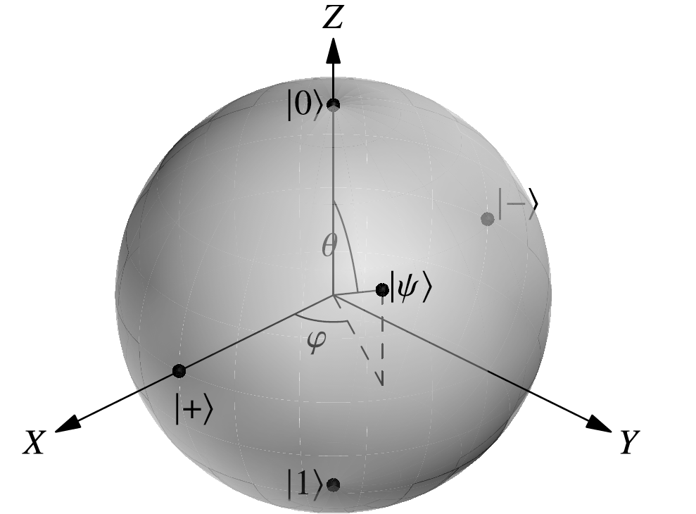
Notice that runs from to  to cover the whole range from the top to the bottom of the sphere. This is why we used in the representation of our preceding qubit. We only needed to get up to
  for our angles in the sines and cosines!
In the Bloch sphere, is mapped to the North pole and to the South pole. In general, states that are orthogonal with respect to the inner product are antipodal on the sphere. For instance, and both lie on the equator, but on opposite points of the sphere. As we already know, the gate takes to and to , but leaves and unchanged, at least up to an irrelevant global phase. In fact, this means that the gate acts like a rotation of radians around the axis of the Bloch sphere…, so now you know why we use that name for the gate! In the same manner, and are rotations of radians around the and axes, respectively.
We can generalize this behavior to obtain rotations of any angle around any axis of the Bloch sphere. For instance, for the , , and axes we may define
 = e^{- i\frac{\theta}{2}X} = \cos\frac{\theta}{2}I - i\sin\frac{\theta}{2}X = \begin{pmatrix}
{\cos\frac{\theta}{2}} & {- i\sin\frac{\theta}{2}} \\
{- i\sin\frac{\theta}{2}} & {\cos\frac{\theta}{2}} \\
\end{pmatrix},")
 = e^{- i\frac{\theta}{2}Y} = \cos\frac{\theta}{2}I - i\sin\frac{\theta}{2}Y = \begin{pmatrix}
{\cos\frac{\theta}{2}} & {- \sin\frac{\theta}{2}} \\
{\sin\frac{\theta}{2}} & {\cos\frac{\theta}{2}} \\
\end{pmatrix},")
 = e^{- i\frac{\theta}{2}Z} = \cos\frac{\theta}{2}I - i\sin\frac{\theta}{2}Z = \begin{pmatrix}
e^{- i\frac{\theta}{2}} & 0 \\
0 & e^{i\frac{\theta}{2}} \\
\end{pmatrix} \equiv \begin{pmatrix}
1 & 0 \\
0 & e^{i\theta} \\
\end{pmatrix},")
where we use the  symbol for equivalent action up to a global phase. Notice that
  \equiv X") ,
,  \equiv Y") ,
,  \equiv Z") ,
,  \equiv S") , and
, and  \equiv T") .
.
Exercise 1.7
Check these equivalences by substituting the angles in the definitions of  ,
,  , and
, and  .
.
In fact, it can be proved (see, for instance, the book by Nielsen and Chuang [69]) that for any one-qubit gate there exists a unit vector ") and an angle such that
and an angle such that
.")
For example, choosing  and
and  \right.") we can obtain the Hadamard gate, for it holds that
we can obtain the Hadamard gate, for it holds that
.")
Additionally, it can also be proved that, again for any one-qubit gate , there exist three angles ,  , and
, and  such that
R_{Y}(\beta)R_{Z}(\gamma).")
In fact, you can obtain such a decomposition for any two rotation axes as long as they are not parallel, not just for and .
Moreover, in some quantum computing architectures (including the ones used by companies such as IBM), it is common to use a universal one-qubit gate, called the -gate, that depends on three angles and is able to generate any other one-qubit gate. Its matrix is
 = \begin{pmatrix}
{\cos\frac{\theta}{2}} & {- e^{i\lambda}\sin\frac{\theta}{2}} \\
{e^{i\varphi}\sin\frac{\theta}{2}} & {e^{i{({\varphi + \lambda})}}\cos\frac{\theta}{2}} \\
\end{pmatrix}.")
Exercise 1.8
Show that ") is unitary. Check that
is unitary. Check that  = U(\theta, - \pi\slash 2,\pi\slash 2) \right.") , that
, that  = U(\theta,0,0)") and that, up to a global phase,
and that, up to a global phase,  = R_{Z}(0,0,\theta)") .
.
All these observations about how to construct one-qubit gates from rotations and parametrized families will be very important when we talk about variational forms and feature maps in Chapter 9, Quantum Support Vector Machines, and Chapter 10, Quantum Neural Networks, and also to construct controlled gates later in this chapter.
1.3.5 Hello, quantum world!
To put together everything that we have learned, we are going to create our very first complete quantum circuit. It looks like this:

It doesn't seem very impressive, but let's analyze it part by part. As you know, following convention, the initial state of our qubit is assumed to be , so that's what we have before we do anything. Then we apply the gate, so the state changes to . Finally, we measure the qubit. The probability of obtaining will be  , and that of getting will also be
  , so we have created a circuit that — at least in theory — generates random bits following a perfectly uniform distribution.
To learn more…
Unbiased uniform bit distributions are of great relevance for multiple applications in simulation, cryptography, and even online gambling games. As we will learn in Chapter 2, The Tools of the Trade, current quantum computers deviate from this equilibrium because they are affected by noise and gate and measurement errors. However, protocols to extract perfect random bits even with noisy quantum computers have been proposed and could become one of the first practical applications of quantum computing (see, for instance, the paper by Acín and Masanes [3]).
We can modify the previous circuit to obtain any distribution over and that we desire. If we want the probability of measuring to be  , we just need to consider
  and the following circuit:

Exercise 1.9
Check that, with the preceding circuit, the state before measurement is  and, hence, the probability of measuring is
  and that of measuring is
  .
.
For now, this is all that we need to know about one-qubit states, gates, and measurements. Let us move on to two-qubit systems, where the mysteries of entanglement are awaiting to be revealed!
1.4 Working with two qubits and entanglement
Now that we have mastered the inner workings of solitary qubits, we are ready to up the ante. In this section, we will learn about systems of two qubits and how they can become entangled. We will first define the mathematical representation of two-qubit systems and how we can measure them. After that, we will study different quantum gates that can act on two qubits at once and we will have a look at some of their very interesting and slightly puzzling properties. We will conclude with a simple but enlightening example of a two-qubit circuit. We promise that the ride is going to be amazing!
1.4.1 Two-qubit states
So far, we have worked with qubits in isolation. But the real power of quantum computing cannot be unleashed unless qubits can talk to each other. We will start by considering the simplest case of quantum systems in which there is qubit interaction: two-qubit systems.
Of course, in a two-qubit system, each of the qubits can be in state or in state . Thus, for the two qubits, we have four possible combinations: both are in state , the first one is in state and the second one in state , the first one is in state and the second one in state , or both are in state . These four possibilities form a basis (called the computational basis) of a  -dimensional space and we denote them, respectively, by

Here,  is the symbol for the tensor product. The tensor product of two column vectors is defined by

Hence, the four basis states can be represented by four-dimensional column vectors given by

Usually, we omit the symbol and just write

or

or even

Obviously, in this last case, the number of qubits that we are using must be clear from the context in order not to mistake the state of a one-qubit system with the state of a two-qubit system — or, as we will see soon, any other multi-qubit system!
As we have mentioned, these four states constitute a basis of the vector space of possible states for a two-qubit system. The general expression for the state of such a system is

where  ,
,  ,
,  , and
, and  are complex numbers (called amplitudes, remember?) such that
  .
.
If we measure in the computational basis both qubits at this generic state that we are considering, we will obtain  with probability
  ,
,  with probability
  ,
,  with probability
  , and
, and  with probability
  . In all those cases, the state will collapse to the state corresponding to the outcome of the measurement, just as with one-qubit systems.
Let's now say that we only measure one of the qubits. What happens then? Suppose that we measure the first qubit. Then, the probability of obtaining will be  , which is the sum of the probabilities of all the outcomes in which the first qubit can be . If we measure the first qubit and the result turns out to be , the system will not collapse completely, but it will remain in the state

where we have divided by  to keep the state normalized. The situation in which the result of the measurement is is analogous.
Exercise 1.10
Derive the formulas for the probability of measuring on the first qubit in a general two-qubit state and for the state of the system after the measurement.
Dirac notation is also useful to compute inner products of two-qubit states. We only need to notice that
\left( {\left| \varphi_{1} \right\rangle \otimes \left| \varphi_{2} \right\rangle} \right) = \left\langle \psi_{1} \middle| \varphi_{1} \right\rangle\left\langle \psi_{2} \middle| \varphi_{2} \right\rangle,")
apply distributivity and remember to conjugate the complex coefficients when obtaining a bra from a ket.
Then, for instance, we can notice that the inner product of  and
and  is
is
\left( {\frac{1}{\sqrt{2}}\left| {00} \right\rangle + \frac{1}{\sqrt{2}}\left| {11} \right\rangle} \right) = \qquad} & & \qquad \\
& {\quad\frac{4}{5\sqrt{2}}\left\langle 01 \middle| 00 \right\rangle + \frac{4}{5\sqrt{2}}\left\langle 01 \middle| 11 \right\rangle - \frac{3i}{5\sqrt{2}}\left\langle 11 \middle| 00 \right\rangle - \frac{3i}{5\sqrt{2}}\left\langle 11 \middle| 11 \right\rangle = \qquad} & & \qquad \\
& {\quad\frac{4}{5\sqrt{2}}\left\langle 0 \middle| 0 \right\rangle\left\langle 1 \middle| 0 \right\rangle + \frac{4}{5\sqrt{2}}\left\langle 0 \middle| 1 \right\rangle\left\langle 1 \middle| 1 \right\rangle - \frac{3i}{5\sqrt{2}}\left\langle 1 \middle| 0 \right\rangle\left\langle 1 \middle| 0 \right\rangle - \frac{3i}{5\sqrt{2}}\left\langle 1 \middle| 1 \right\rangle\left\langle 1 \middle| 1 \right\rangle = - \frac{3i}{5\sqrt{2}},\qquad} & & \qquad \\
\end{array}")
since  and
and  .
.
1.4.2 Two-qubit gates: tensor products
Of course, the operations that we can conduct on two-qubit systems need to be unitary. Thus, two-qubit quantum gates are  unitary matrices that act on 4-dimensional column vectors. The simplest way to construct such matrices is by taking the tensor product of two one-qubit quantum gates. Namely, if we consider two one-qubit gates
  and
and  and two one-qubit states
  and
and  , we can form a two-qubit gate
  that acts on
  as
as
\left( {\left| \psi_{1} \right\rangle \otimes \left| \psi_{2} \right\rangle} \right) = \left( {U_{1}\left| \psi_{1} \right\rangle} \right) \otimes \left( {U_{2}\left| \psi_{2} \right\rangle} \right).")
By linearity, we can extend to any combination of two-qubit states and we can associate a matrix to . In fact, said matrix is given by the tensor product of the matrices associated to and . More concretely, the expression for the tensor product,  , of the matrices
  and
and  is
is

Now it is easy to verify that this operation is indeed unitary and, hence, deserves the name of quantum gate.
Exercise 1.11
Check that, given any pair of unitary matrices and , the inverse of is  and that
 }^{\dagger} = U_{1}^{\dagger} \otimes U_{2}^{\dagger}") .
.
Tensor products of gates occur naturally when we have circuits with two qubits and pairs of individual one-qubit gates are acting on each of them. For instance, in the following circuit, the gate  acts on the two qubits and then it is followed by the gate
  , where is the identity gate:

Exercise 1.12
Explicitly compute the matrices for the gates and .
You may complain that we haven't done anything new so far. And you would be right! In fact, quantum gates that are obtained as the tensor product of one-qubit gates can be seen as operations on isolated qubits that just happen to be applied at the same time. But wait and see! In the next subsection, we will introduce a completely different way of acting on two-qubit systems.
1.4.3 The CNOT gate
By taking tensor products of one-qubit gates, we can only obtain operations that act on each qubit individually. But this just leaves us with a (rather boring) subset of all the possible two-qubit gates. There are many unitary matrices that cannot be written as the tensor product of other simple matrices. In the two-qubit case, probably the most important one is the controlled-NOT (or controlled- ) gate, usually called the CNOT gate, given by the unitary matrix

It is illuminating to see how this gate acts on the elements of the two-qubit computational basis. As you can easily check, we get

This means that the value of the second qubit is flipped if and only if the value of the first qubit is . Or, to put it in other words, the application of a NOT gate on the second qubit (that we call the target) is controlled by the first qubit. Now the name of this gate makes much more sense, doesn't it?
In a quantum circuit, the CNOT gate is represented as follows:

Notice that the control qubit is indicated by a solid black circle and the target qubit is indicated by the  symbol (the symbol for an gate can also be used instead of ).
Sometimes, technical difficulties restrict the number of CNOT gates that can be actually implemented on a quantum computer. For instance, on a certain quantum chip you may have the possibility of applying a CNOT gate targeting qubit and controlled by qubit , but not the other way around. If you find yourself in such a situation, there's no need to panic. If you use the circuit

you are effectively applying a CNOT gate with target in the top qubit and control in the bottom one. And that's how you can save the day!
The CNOT gate can also be used to interchange or swap the states of two qubits, by using the following circuit:

Exercise 1.13
Check these equivalences in two different ways: by computing the matrices of the circuits and by obtaining the result of using them with qubits in states  ,
,  ,
,  , and
, and  .
.
In any case, the most prominent use of the CNOT gate is, without a doubt, the ability to create entanglement, an intriguing property of quantum systems that we will study next.
1.4.4 Entanglement
Oddly enough, in order to define when a quantum system is entangled, we first need to define when it is not entangled. We say that a state is a product state if it can be written as the tensor product of two other states and , each of at least one qubit,
as in

If is not a product state, we say that it is entangled.
For example, is a product state, because we know that it is just another way of writing  . Also,
 ") is a product state, because we can factor on the second qubit to obtain
is a product state, because we can factor on the second qubit to obtain
 = \left( {\frac{1}{\sqrt{2}}\left( {\left| 0 \right\rangle + \left| 1 \right\rangle} \right)} \right)\left| 0 \right\rangle.")
On the other hand, ") is an entangled state. No matter how hard you try, it is impossible to write it as a product of two one-qubit states. Suppose, for sake of contradiction, that it were possible. Then, you would have
is an entangled state. No matter how hard you try, it is impossible to write it as a product of two one-qubit states. Suppose, for sake of contradiction, that it were possible. Then, you would have
} & {= \left( {a\left| 0 \right\rangle + b\left| 1 \right\rangle} \right)\left( {c\left| 0 \right\rangle + d\left| 1 \right\rangle} \right)\qquad} & & \qquad \\
& {= ac\left| {00} \right\rangle + ad\left| {01} \right\rangle + bc\left| {01} \right\rangle + bd\left| {11} \right\rangle.\qquad} & & \qquad \\
\end{array}")
But this forces  to be , because we have no component in
 ") . Then, either
. Then, either  , in which case
  is , or
  , from which
  follows. In both cases, it is impossible to reach the equality that we needed. Thus, it follows that the state is entangled.
Exercise 1.14
Is ") entangled? And what about
entangled? And what about ") ?
?
When measured, entangled states can show correlations that go beyond what can be explained with classical physics. For instance, if we have the entangled state and we measure the first qubit, we can obtain or , each with probability . However, if we measure the second qubit afterwards, the result will be completely determined by the value obtained when measuring the first qubit and, in fact, will be exactly the same. If we invert the order and measure first the second qubit, then the result will be or , with equal probability. But, in this case, the result of a subsequent measurement of the first qubit will be completely determined!
This still happens even if we separate the two qubits thousands of light years apart, as if one qubit could somehow know what the result of measuring the other qubit was. This curious behavior haunted many physicists during the 20th century, including Albert Einstein, who called it a "spooky action at a distance" (see [34]). Nevertheless, the effects of entanglement have been repeatedly demonstrated in uncountable experiments (in fact, the Nobel Prize in Physics 2022 was awarded to Alain Aspect, John F. Clauser, and Anton Zeilinger, pioneers in studying and testing this phenomenon in practice [10, 25, 41, 19]). And, very importantly for us, entanglement is one of the most powerful resources available in quantum computing.
But entanglement is, by no means, the only puzzling feature of qubit systems. In the next subsection, we are going to mathematically prove that copying quantum information, an operation that you may have taken for granted, is not possible in general. These qubits are, indeed, full of surprises!
1.4.5 The no-cloning theorem
Another peculiar property of quantum systems is that, in general, they don't allow us to copy information. Surprising as this may seem, it is just an easy consequence of the linearity of quantum gates. To show why, let us be more precise about what we would need in order to copy information, for instance with just two qubits. We would like to have a two-qubit quantum gate that will be able to copy the first qubit into the second. That is, for any given quantum state , we would need

Then,  and
and  and, by linearity,
} \right) = \frac{1}{\sqrt{2}}\left( {U\left| {00} \right\rangle + U\left| {10} \right\rangle} \right) = \frac{1}{\sqrt{2}}\left( {\left| {00} \right\rangle + \left| {11} \right\rangle} \right).")
We should highlight that the state that we have obtained is entangled, as we proved in the previous subsection.
Nevertheless, notice that, in our original state, we can factor the second out to obtain
 = \left( \frac{\left| 0 \right\rangle + \left| 1 \right\rangle}{\sqrt{2}} \right)\left| 0 \right\rangle.")
Then, in virtue of the action of , we should have
} \right) = U\left( {\left( \frac{\left| 0 \right\rangle + \left| 1 \right\rangle}{\sqrt{2}} \right)\left| 0 \right\rangle} \right) = \frac{(\left| 0 \right\rangle + \left| 1 \right\rangle)}{\sqrt{2}}\frac{(\left| 0 \right\rangle + \left| 1 \right\rangle)}{\sqrt{2}},")
which is a product state. However, we had obtained earlier that ) = \sqrt{\left. 1\slash 2 \right.}(\left| {00} \right\rangle + \left| {11} \right\rangle)") , which is entangled! This contradiction implies that, alas, no such exists.
, which is entangled! This contradiction implies that, alas, no such exists.
This remarkable result is called the no-cloning theorem and we should explain its meaning in a little more detail. On the one hand, notice that this does not imply that we cannot copy classical information. In fact, if is just or , we can easily achieve  by taking to be the CNOT gate. On the other hand, the theorem applies to unknown states . If we know what is — that is, if we know a circuit that prepares starting from — then, of course, we can create as many independent copies of it as we want. However, if is handed to us without any additional information about its state, the no-cloning theorem shows that we cannot replicate its state in general.
To learn more…
The no-cloning theorem plays an important role in the security of quantum key distribution protocols such as the famous BB84, introduced in 1984 by Bennett and Brassard [13].
After this brief detour, let's return to our study of two-qubit quantum gates. In the next subsection, we will show how to construct many interesting two-qubit unitary operations whose action is controlled by one of their inputs.
1.4.6 Controlled gates
You may be wondering if, in addition to a controlled- (or CNOT) gate, there are also controlled- , controlled-
 , or controlled-
 gates. The answer is a resounding yes and, in fact, for any quantum gate , it is possible to define a controlled- (or, simply,
  ) gate whose action on the computational basis is

Exercise 1.15
Check that the matrix of  is
is

where }_{i,j = 1}^{2}") is the matrix of . Check also that is unitary. What is the adjoint of ?
is the matrix of . Check also that is unitary. What is the adjoint of ?
The circuit representation of a gate is similar to the one that we use for the CNOT gate, namely
 ,
,
where the solid black circle indicates the control and the box with inside indicates the target.
Constructing a controlled gate is simpler than it seems, provided your quantum computer already implements rotation gates and the two-qubit CNOT gate. In fact, from the decomposition in rotations that we mentioned at the end of Section 1.3.4, it can be proved (see the book by Nielsen and Chuang [69, Corollary 4.2]) that any one-qubit quantum gate can be written in the form

for some angle and gates , , and  such that
  . Then, the following circuit implements :

Sometimes, though, constructing a controlled gate is much easier. For instance, it can be shown that a controlled- gate can be obtained from a controlled- and two gates, as shown in the identity of the following circuits:


Exercise 1.16
Prove the preceding equivalence.
We now have everything we need in order to construct our first two-qubit quantum circuit. Let's get those qubits entangled!
1.4.7 Hello, entangled world!
To finish up with our study of two-qubit systems, let us show how to create entangled states with the help of the CNOT gate. Consider the following circuit:

Initially, the state of the system is . After we apply the gate, we get into the state . Finally, when we apply the CNOT gate, the state changes to , which, as we proved in Section 1.4.4, is indeed an entangled state.
The state is known as a Bell state, of which there are four. The other three are ") ,
, ") , and
, and ") . All of them are entangled, and they can be prepared with circuits similar to the preceding one.
. All of them are entangled, and they can be prepared with circuits similar to the preceding one.
Exercise 1.17
Show that all four Bell states are entangled. Obtain circuits to prepare them. Hint: you can use and gates after the CNOT in the preceding circuit.
We are now ready for the big moment. In the next section, we will finally learn how to work with not just one or two qubits, but with as many as we can get in our quantum computers.
1.5 Working with multiple qubits and universality
Now that we have mastered working with two-qubit systems, it will be fairly straightforward to generalize all the notions that we have been studying to the case in which the number of qubits in our circuits is arbitrarily big. You know the drill: we will start by defining, mathematically, what a multi-qubit system is, we will then learn how to measure it and, finally, we will introduce quantum gates that act on many qubits at the same time.
1.5.1 Multi-qubit systems
With all that we have learned so far, it will now be very easy to understand how to work with multi-qubit systems.
As you may have already deduced, if we have  qubits, the states that constitute the computational basis are

We usually omit the symbol to write

or

or simply

Important note
When using the  notation for basis states, the total number of qubits must be clear from context. Otherwise, a state like, for example,
  might mean either ,
  ,
,  , or any string with leading zeroes and ending in …and that would be an intolerable ambiguity!
Of course, a generic state of the system will then be of the form

subject to the only condition that the amplitudes  should be complex numbers such that
  . Our dear old friend, the normalization condition!
To learn more…
Notice that the number of parameters describing the general state of an -qubit system is exponential in . For highly entangled states, we do not know how to represent all this information in a more succinct way and it is strongly suspected that it is not possible. Part of the power of quantum computing comes from this possibility of implicitly working with  complex numbers by manipulating just qubits.
Exercise 1.18
Check that the basis state  is represented by a -dimensional column vector whose
  -th component is 1, while the rest are 0 (Hint: Use, repeatedly, the expression for the tensor product of column vectors that we discussed in Section 1.4.1 and the fact that the tensor product is associative). Deduce that any -qubit state can be represented by a -dimensional column vector with unit length.
If we decide to measure all the qubits of the system in the computational basis, we will obtain  with probability
  . If that is the case, then the state will collapse to
  . But if we only measure one of the qubits, say the -th one, then we will obtain with probability

where  is the set of numbers whose -th bit is . In this scenario, the state of the system after measuring would be

Exercise 1.19
Derive the formulas for the case in which the result of the measurement is .
Exercise 1.20
What is the probability of getting when we measure the second qubit of \left| {100} \right\rangle + (1\slash 2)\left| {010} \right\rangle + \sqrt{\left. 1\slash 2 \right.}\left| {001} \right\rangle \right.") ? What will the state be after the measurement if we indeed get ?
? What will the state be after the measurement if we indeed get ?
Computing inner products of -qubit systems in Dirac notation is very similar to doing it with two-qubit systems. The procedure is analogous to the one we showed in Section 1.4.1, but taking into account that
\left( {\left| \varphi_{1} \right\rangle \otimes \ldots \otimes \left| \varphi_{n} \right\rangle} \right) = \left\langle \psi_{1} \middle| \varphi_{1} \right\rangle\ldots\left\langle \psi_{n} \middle| \varphi_{n} \right\rangle.")
Exercise 1.21
Compute the inner product of  and
and  , where
  and
and  are both binary strings of length . Use your result to prove that
  is, indeed, an orthonormal basis.
Exercise 1.22
Compute the inner product of the states ") and
and  \right.") .
.
We can now turn to the question of how to operate on many qubits at once. Let's define multi-qubit gates!
1.5.2 Multi-qubit gates
Since -qubit states are represented by -dimensional column vectors, -qubit gates can be identified with  unitary matrices. Similar to the two-qubit case, we can construct -qubit gates by taking the tensor product of gates on a smaller number of qubits. Namely, if is an
  -qubit gate and is an
  -qubit gate, then is an
 ") -qubit gate and its matrix is given by the tensor product of the matrices and .
-qubit gate and its matrix is given by the tensor product of the matrices and .
To learn more…
The expression for the tensor product of two matrices and is

However, there are -qubit gates that cannot be constructed as tensor products of smaller gates. One such example is the Toffoli or CCNOT gate, a three-qubit gate that acts on the computational basis as
} \right\rangle,")
where is the XOR function and  is the symbol for the AND Boolean function. Thus, CCNOT applies a doubly controlled (in this case, by the first two qubits) NOT gate to the third qubit — hence the name!
Exercise 1.23
Obtain the matrix for the CCNOT gate and verify that it is unitary.
The Toffoli gate is important because, using it and with the help of auxiliary qubits, we can construct any classical Boolean operator. For instance,  (where
  is the negation of ) and
  . This shows that, with quantum circuits, we can simulate the behavior of any classical digital circuit at the cost of using some additional ancillary qubits, since any Boolean function can be built with just negations and conjunctions. This is somewhat surprising, because we know that all quantum gates are invertible, while not all Boolean functions are. It then follows that we could make all of our digital circuits reversible just by implementing a classical version of the Toffoli gate!
We will not be studying any other concrete examples of gates that act on three (or more!) qubits because, in fact, we can simulate their behavior with circuits that only use one- and two-qubit gates. Keep on reading to know how!
1.5.3 Universal gates in quantum computing
Current quantum computers can't implement every possible quantum gate. Instead, they rely on universality results that show how any unitary operation can be decomposed as a circuit that uses a reduced set of primitive gates. In previous sections, we mentioned, for instance, that any one-qubit gate can be obtained by using just and rotations. It turns out that similar results exist for the general case of -qubit quantum gates.
To us, it will be important to know that, for any unitary operation, we can construct a circuit that implements it using only one-qubit gates and the CNOT gate. For this reason, we say that those gates are universal — in the same sense that, for example, negation and conjunction are universal for Boolean logic. This fact will be crucial for our study of feature maps and variational forms in connection to quantum neural networks and other quantum machine learning models.
To learn more…
In addition to one-qubit gates plus CNOT, there are many other sets of universal gates. For instance, it can be shown that the three gates , , and CNOT can be used to approximate any unitary operation to any desired accuracy — and they are universal in that sense. See Section 4.5 of the book by Nielsen and Chuang [69] for proofs of these facts and for more examples of universal gate sets.
To illustrate how CNOT and one-qubit gates can be used to implement any other quantum gate, the following circuit shows a possible decomposition of the Toffoli gate targeting the top qubit:
 .
.
Exercise 1.24
Verify that the preceding circuit implements the Toffoli gate by checking its action on the states of the computational basis.
This concludes our review of the fundamentals of quantum computing. We've come a long way since the beginning of this chapter, but by now we have mastered all the mathematics that we will need in order to study quantum machine learning and quantum optimization algorithms. Soon, we will see all these concepts in action!
Summary
In this chapter, we have introduced the quantum circuit model and the main concepts that it relies on: qubits, gates, and measurements. We have started by studying the most humble circuits, those that only have one or two qubits, but we have used our experience with them to grow all the way up to multi-qubit systems. In the process, we have discovered some powerful properties, such as superposition and entanglement, and we have mastered the mathematics — mainly some linear algebra — needed to work with them.
These notions will be extremely valuable to us, because they make up the language in which we will be describing the quantum algorithms for machine learning and optimization that we will study in the rest of the book. Soon, all the pieces will come together to form a beautiful structure. And we will be able to appreciate it and understand it fully because of the solid foundations that we have acquired by now.
In the next chapter, we will start applying all that we have learned by implementing and running quantum circuits on quantum simulators and on actual quantum computers. We don't know about you, but we are pretty excited!