A simulation model is a tool capable of processing information and data and predicting the responses of a real system to certain inputs, providing effective support for analysis, performance evaluation, and decision-making processes. The term simulation refers to reproducing the behavior of a system. In a simulation, we can use a real model, perhaps in scale, or a numerical model, which reproduces reality using a computer. An example of a real model is a scale model of an airplane, which is then placed in a wind tunnel to run simulated tests to estimate suitable performance measures.

Although, over the years, physicists have developed theoretical laws that we can use to obtain information on the performance of dynamic systems, often, the application of these laws to a real case takes too long. In these cases, it is convenient to construct a numerical simulation model that allows us to simulate the behavior of the system under certain conditions. This elaborated model will allow us to test the functionality of the system in a simple and immediate way, saving considerable resources in terms of time and money.

In this chapter, we’re going to cover the following main topics:

• Introducing simulation models
• Classifying simulation models
• Approaching a simulation-based problem
• Exploring discrete event simulation
• Dynamical systems modeling
• How to run efficient simulations to analyze real-world systems

In this chapter, an introduction to simulation techniques will be discussed. To deal with the topics at hand, it is necessary that you have a basic knowledge of algebra and mathematical modeling.

Simulation uses digital models developed to replicate the characteristics of a system. The system functioning is simulated using probability distributions to randomly generate system events, and statistical observations are obtained from the simulated system. It plays a very important role, especially in the design of a stochastic system and in the definition of its operating procedures.

By not working directly on the real system, many scenarios can be simulated simply by changing the input parameters, thus limiting the costs and reducing time. In this way, it is possible to quickly try alternative policies and design choices and model systems of great complexity by studying their behavior and evolution over time.

Important note

Simulation is used when working on real systems is not convenient due to high costs, technical impossibility, and the non-existence of a real system. The simulation predicts what will happen to the real system if certain inputs are used: changing these input parameters reproduces different scenarios by identifying the most convenient one from various points of view.

Decision-making workflow

In a decision-making process, the starting point is identifying the problem that requires a change and, therefore, a decision. The identified problem is then analyzed to highlight what needs to be studied for the decisions to be made; that is, the relevant elements are chosen, the relationships that bind them are highlighted, and the objectives to be achieved are defined. At this point, a formal model is built, which allows the simulation of the system to understand its behavior and identify the decisions to be made. The following diagram depicts the workflow that allows us to make a decision, starting from the observation of the problem scenario:

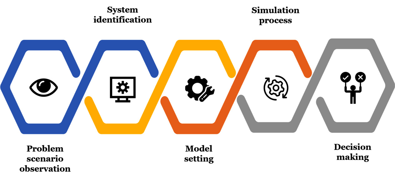
Figure 1.1: Decision-making workflow

The model building is a two-way process:

• Definition of conceptual models
• Continuous interaction between the model and reality by comparison

In addition, learning also has a participatory characteristic: it proceeds through the involvement of different actors. The models also allow you to analyze and propose organized actions so that you can modify the current situation and produce the desired solution.

Comparing modeling and simulation

To start, we will clarify the differences between modeling and simulation. A model is a representation of a physical system, while simulation is the process of seeing how a model-based system would work under certain conditions.

Modeling is a design methodology based on producing a model implementation for a system and representing its functionality. In this way, it is possible to predict the system’s behavior and the effects of variations or modifications that are made to it. Even if the model is a simplified system representation, it must still be close enough to the functional nature of the real system, but without becoming too complex and difficult to handle.

Important note

Simulation is the process that puts the model into operation and allows you to evaluate its behavior under certain conditions. Simulation is a fundamental tool for modeling because, without necessarily resorting to physical prototyping, the developer can verify the functionality of the modeled system with the project specifications.

In the simulation, the system is studied by reproducing all possible operating conditions, even the impossible ones, without worrying about the costs involved in such experiments.

The simulation is the transposition in logical-mathematical-procedural terms of a conceptual model of the real system. This conceptual model can be defined as the set of processes that take place in the evaluated system and whose whole allows us to understand the operating logic of the system itself.

Pros and cons of simulation modeling

Simulation is a tool that’s widely used in a variety of fields, from operational research to the application industry. This technique can be made successful by it overcoming the difficulties that each complex procedure contains. The following are the pros and cons of simulation modeling. Let’s start with the concrete advantages that can be obtained from the use of simulation models (pros):

• It reproduces the behavior of a system in reference to situations that cannot be directly experienced
• It represents real systems, even complex ones, while also considering the sources of uncertainty
• It requires limited resources in terms of data
• It allows experimentation in a limited time
• The models that are obtained are easily interpretable

As anticipated, since it is a technique capable of reproducing complex scenarios, it has some limitations (cons):

• The simulation provides indications of the behavior of the system but not exact results
• The analysis of the output of a simulation could be complex, and it could be difficult to identify which may be the best configuration
• The implementation of a simulation model could be laborious and, moreover, it may take a long time to carry out a significant simulation
• The results that are returned by the simulation depend on the quality of the input data: it cannot provide accurate results in the case of inaccurate input data
• The complexity of the simulation model depends on the complexity of the system it intends to reproduce

Nevertheless, simulation models represent the best solution for the analysis of complex scenarios.

Simulation modeling terminology

In this section, we will analyze the elements that make up a model and those that characterize a simulation process. We will give a brief description of each so that you understand their meaning and the role they play in the numerical simulation process.

System

The context of an investigation is represented through a system, that is, the set of elements that interact with each other. The main problem linked to this element concerns the system boundaries, that is, which elements of reality must be inserted into the system that it represents and which are left out, and the relationships that exist between them.

State variables

A system is described in each instant of time by a set of variables. These are called state variables. For example, in the case of a weather system, the temperature is a state variable. In discrete systems, the variables change instantly at precise moments of time that are finite. In continuous systems, the variables vary in terms of continuity with respect to time.

Events

An event is defined as any instantaneous event that causes the value of at least one of the status variables to change. The arrival of a blizzard for a weather system is an event, as it causes the temperature to drop suddenly. There are both external events and internal events.

Parameters

Parameters represent essential terms when building a model. They are adjusted during the model simulation process to ensure that the results are brought into the necessary convergence margins. They can be modified iteratively through sensitivity analysis or in the model calibration phase.

Calibration

Calibration represents the process by which the parameters of the model are adjusted to adapt the results to the data observed in the best possible way. When calibrating the model, we try to obtain the best possible accuracy. A good calibration requires eliminating, or minimizing, errors in data collection and choosing a theoretical model that is the best possible description of reality. The choice of model parameters is decisive and must be done in such a way as to minimize the deviation of its results when applied to historical data.

Accuracy

Accuracy is the degree of correspondence of the simulation result that can be inferred from a series of calculated values with the actual data, that is, the difference between the average modeled value and the true or reference value. Accuracy, when calculated, provides a quantitative estimate of the quality expected from a forecast. Several indicators are available to measure accuracy. The most widely used ones are mean absolute error (MAE), mean absolute percentage error (MAPE), and mean square error (MSE).

Sensitivity

The sensitivity of a model indicates the degree to which the model’s outputs are affected by changes in the selected input parameters. Sensitivity analysis identifies the sensitive parameters for the output of the model. It allows us to determine which parameters require further investigation so that we have a more realistic evaluation of the model’s output values. Furthermore, it allows us to identify which parameters are not significant for the generation of a certain output and, therefore, can possibly be eliminated from the model. Finally, it tells us which parameters should be considered in a possible and subsequent analysis of the uncertainty of the output values provided by the model.

Validation

This is the process that verifies the accuracy of the proposed model. The model must be validated to be used as a tool to support decisions. It aims to verify whether the model that’s being analyzed corresponds conceptually to our intentions. The validation of a model is based on the various techniques of multivariate analysis, which, from time to time, study the variability and interdependence of attributes within a class of objects.

Now that we have understood what simulation models are and the various pros, cons, and features they have, we will learn how to classify them in the next section.

Simulation models can be classified according to different criteria. The first distinction is between static and dynamic systems. So, let’s see what differentiates them.

Comparing static and dynamic models

A system is an object with a finite number of degrees of freedom that evolves over time according to a deterministic law. A system can be represented as a black box that can be stimulated by a stress (input) x (t) and that produces an effect (output) y (t). The behavior of the system is fully described by the following equation:

Static models are the representation of a system in an instant of time or representative models of a system in which the time variable plays no role. An example of a static simulation is a Monte Carlo model.

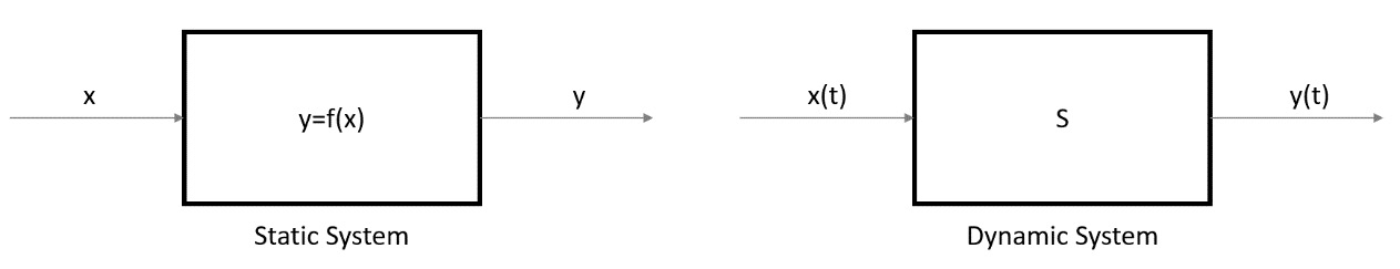
Figure 1.2: Static versus dynamic system representation

Dynamic models, on the other hand, describe the evolution of the system over time. In the simplest case, the state of the system at time t is described by a function x (t). For example, in population dynamics, x (t) represents the population present at time t. The equation that regulates the system is dynamic: it describes the instantaneous variation of the population or the variation in fixed time intervals.

Comparing deterministic and stochastic models

A model is deterministic when its evolution, over time, is uniquely determined by its initial conditions and characteristics. These models do not consider random elements and lend themselves to be solved with exact methods that are derived from mathematical analysis. In deterministic models, the output is well determined once the input data and the relationships that make up the model have been specified, despite the time required for data processing being particularly long. For these systems, the transformation rules univocally determine the change of state of the system. Examples of deterministic systems can be observed in some production and automation systems.

Stochastic models, on the other hand, can be evolved by inserting random elements into the evolution. These are obtained by extracting them from statistical distributions. Among the operational characteristics of these models, there is not just one relationship that fits all. There are also probability density functions, which means there is no one-to-one correspondence between the data and system history.

A final distinction is based on how the system evolves over time: therefore, we distinguish between continuous and discrete simulation models.

Comparing continuous and discrete models

Continuous models represent systems in which the state of the variables changes continuously as a function of time. For example, a car moving on a road represents a continuous system since the variables that identify it, such as position and speed, can change continuously with respect to time.

In discrete models, the system is described by an overlapping sequence of physical operations interspersed with inactivity pauses. These operations begin and end in well-defined instances (events). The system undergoes a change of state when each event occurs, remaining in the same state throughout the interval between the two subsequent events. This type of operation is easy to treat with the simulation approach.

Important note

The stochastic, deterministic, continuous, or discrete nature of a model is not its absolute property and depends on the observer’s vision of the system itself. This is determined by the objectives and the method of study, as well as by the experience of the observer.

Now that we’ve analyzed the different types of models in detail, we will learn how to develop a numerical simulation model.

To tackle a numerical simulation process that returns accurate results, it is crucial to rigorously follow a series of procedures that partly precede and partly follow the actual modeling of the system. We can separate the simulation process workflow into the following individual steps:

1. Problem analysis
2. Data collection
3. Setting up the simulation model
4. Simulation software selection
5. Verification of the software solution
6. Validation of the simulation model
7. Simulation and analysis of results

To fully understand the whole simulation process, it is essential to analyze in depth the various phases that characterize a study based on simulation.

Problem analysis

In this initial step, the goal is to understand the problem by trying to identify the aims of the study and the essential components, as well as the performance measures that interest them. Simulation is not simply an optimization technique, and therefore, there is no parameter that needs to be maximized or minimized. However, there is a series of performance indices whose dependence on the input variables must be verified. If an operational version of the system is already available, the work is simplified as it is enough to observe this system to deduce its fundamental characteristics.

Data collection

This represents a crucial step in the whole process since the quality of the simulation model depends on the quality of the input data. This step is closely related to the previous one. In fact, once the objective of the study has been identified, data is collected and subsequently processed. Processing the collected data is necessary to transform it into a format that can be used by the model. The origin of the data can be different: sometimes, the data is retrieved from company databases, but often, direct measurements in the field must be made through a series of sensors that, in recent years, have become increasingly smart. These operations weigh down the entire study process, thus lengthening their execution times.

Setting up the simulation model

This is the most crucial step of the whole simulation process; therefore, it is necessary to pay close attention to it. To set up a simulation model, it is necessary to know the probability distributions of the variables of interest. In fact, to generate various representative scenarios of how a system works, it is essential that a simulation generates random observations from these distributions.

For example, when managing stocks, the distribution of the product being requested and the distribution of time between an order and the receipt of the goods is necessary. On the other hand, when managing production systems with machines that can occasionally fail, it will be necessary to know the distribution of time until a machine fails and the distribution of repair times.

If the system is not already available, it is only possible to estimate these distributions by deriving them, for example, from the observation of similar, already existing systems. If, from an analysis of the data, it is seen that this form of distribution approximates a standard type distribution, the standard theoretical distribution can be used by carrying out a statistical test to verify whether the data can be well represented by that probability distribution. If there are no similar systems from which observable data can be obtained, other sources of information must be used, such as machine specifications, instruction manuals for the same, and experimental studies.

As we’ve already mentioned, constructing a simulation model is a complex procedure. Referring to simulating discrete events, constructing a model involves the following steps:

1. Defining the state variables
2. Identifying the values that can be taken by the state variables
3. Identifying the possible events that change the state of the system
4. Realizing a simulated time measurement, that is, a simulation clock, that records the flow of simulated time
5. Implementing a method for randomly generating events
6. Identifying the state transitions generated by events

After following these steps, we will have the simulation model ready for use. At this point, it will be necessary to implement this model in a dedicated software platform; let’s see how.

Simulation software selection

The choice of the software platform that you will perform the numerical simulation on is fundamental for the success of the project. In this regard, we have several solutions that we can adopt. This choice will be made based on our knowledge of programming. Let’s see what solutions are available:

• Simulators: These are application-oriented packages for simulation. There are numerous interactive software packages for simulation, including MATLAB, COMSOL Multiphysics, Ansys, SolidWorks, Simulink, Arena, AnyLogic, and SimScale. These pieces of software represent excellent simulation platforms whose performance differs based on the application solutions provided. These simulators allow us to elaborate on a simulation environment using graphic menus without the need to program.

They are easy to use and many of them have excellent modeling capabilities, even if you just use their standard features. Some of them provide animations that show the simulation in action, which allows you to easily illustrate the simulation to non-experts. The limitations presented by this software solution are the high costs of the licenses, which can only be faced by large companies, and the difficulty in modeling solutions that have not been foreseen by the standards.

• Simulation languages: A more versatile solution is offered by the different simulation languages available. There are solutions that facilitate the task of the programmer who, with these languages, can develop entire models or sub-models with a few lines of code that would otherwise require much longer drafting times, with a consequent increase in the probability of error. An example of a simulation language is the general-purpose simulation system (GPSS). This is a generic programming language that was developed by IBM in 1965. In it, a simulation clock advances in discrete steps, modeling a system as transactions enter the system and are passed from one service to another. It is mainly used as a process flow-oriented simulation language and is particularly suitable for application problems. Another example of a simulation language is SimScript, which was developed in 1963 as an extension of Fortran. SimScript is an event-based scripting language, so different parts of the script are triggered by different events.
• GPSS: A general-purpose programming language is designed to be able to create software in numerous areas of application. They are particularly suitable for the development of system software such as drivers, kernels, and anything that communicates directly with the hardware of a computer. Since these languages are not specifically dedicated to a simulation activity, they require the programmer to work harder to implement all the mechanisms and data structures necessary in a simulator. On the other hand, by offering all the potential of a high-level programming language, they offer the programmer a more versatile programming environment. In this way, you can develop a numerical simulation model perfectly suited to the needs of the researcher. In this book, we will use this solution by devoting ourselves to programming with Python. This software platform offers a series of tools that have been created by researchers from all over the world that make the elaboration of a numerical modeling system particularly easy. In addition, the open source nature of the projects written in Python makes this solution particularly inexpensive.

Now that we’ve chosen the software platform we’re going to use and have elaborated on the numerical model, we need to verify the software solution.

Verification of the software solution

In this phase, a check is carried out on the numerical code. This is known as debugging, which consists of ensuring that the code correctly follows the desired logical flow without unexpected blocks or interruptions. The verification must be provided in real time during the creation phase because correcting any concept or syntax errors becomes more difficult as the complexity of the model increases.

Although verification is simple in theory, debugging large-scale simulation code is a difficult task due to virtual competition. The correctness or otherwise of executions depends on time, as well as on the large number of potential logical paths. When developing a simulation model, you should divide the code into modules or subroutines in order to facilitate debugging. It is also advisable to have more than one person review the code, as a single programmer may not be a good critic. In addition, it can be helpful to perform the simulation when considering a large variety of input parameters and checking that the output is reasonable.

Important note

One of the best techniques that can be used to verify a discrete-event simulation program is one based on tracking. The status of the system, the content of the list of events, the simulated time, the status variables, and the statistical counters are shown after the occurrence of each event and then compared with hand-made calculations to check the operation of the code.

A track often produces a large volume of output that needs to be checked event by event for errors. Possible problems may arise, including the following:

• There may be information that hasn’t been requested by the analyst
• Other useful information may be missing, or a certain type of error may not be detectable during a limited debugging run

After the verification process, it is necessary to validate the simulation model.

Validation of the simulation model

In this step, it is necessary to check whether the model that has been created provides valid results for the system in question. We must check whether the performance measurements of the real system are well approximated by the measurements generated by the simulation model. A simulation model of a complex system can only approximate it. A simulation model is always developed for a set of objectives. A model that’s valid for one purpose may not be valid for another.

Important note

Validation checks that the level of accuracy between the model and the system is respected. It is necessary to establish whether the model adequately represents the behavior of the system. The value of a model can only be defined in relation to its use. Therefore, validation is a process that aims to determine whether a simulation model accurately represents the system for the set objectives.

In this step, the ability of the model to reproduce the real functionality of the system is ascertained; that is, it is ensured that the calibrated parameters, relative to the calibration scenario, can be used to correctly simulate other system situations. Once the validation phase is over, the model can be considered transferable and, therefore, usable for the simulation of any new control strategies and new intervention alternatives. As widely discussed in the literature on this subject, it is important to validate the model parameters that were previously calibrated based on data other than that used to calibrate the model, always with reference to the phenomenon specific to the scenario being analyzed.

Simulation and analysis of results

A simulation is a process that evolves during its realization, and where the initial results help lead the simulation toward more complex configurations. Attention should be paid to some details. For example, it is necessary to determine the transient length of the system before reaching stationary conditions if you want performance measures of the system at full capacity. It is also necessary to determine the duration of the simulation after the system has reached equilibrium. In fact, it must always be kept in mind that a simulation does not produce the exact values of the performance measures of a system since each simulation is a statistical experiment that generates statistical observations regarding the performance of the system. These observations are then used to produce estimates of performance measures. Increasing the duration of the simulation can increase the accuracy of these estimates.

The simulation results return statistical estimates of a system’s performance measures. The fundamental point is that each measurement is accompanied by a confidence interval, within which it can vary. These results could immediately highlight a better system configuration than the others, but more often, more than one candidate configuration will be identified. In this case, further investigations may be needed to compare these configurations.

Now that we’ve analyzed a generalized simulation-based problem, we will learn how to approach a Discrete Event Simulation.

A DES is a dynamic system whose states can assume logical or symbolic values rather than numerical ones. The behavior of the system is characterized by the occurrence of instantaneous events that arise with an irregular timing not necessarily known a priori. The behavior of such systems is described in terms of states and events.

A DES considers the system as a sequence of discrete events over time: each event occurs at a particular instant t and implements a change of state in the system. Therefore, between two consecutive events, it is assumed that there is no change of state, and therefore once the event is concluded at a certain instant t1, it is possible to go directly to the instant of the start of the next event t2.

In DES, the evolutions of the system over time are represented with variables that instantly change value in defined instants of time, included in a well-defined numerical interval, which determines the occurrence of events. The objects in a simulation system of this type are distinct elements, each having its own characteristics that determine its behavior within the model, which are called tokens. Discrete event simulation models are characterized by the following points:

• State variables that take on discrete values
• Transitions from one state to another that occur in discrete moments

To simulate a discrete event model, it is necessary to identify the state variables of the system and the classes of events that give rise to state transitions. Generally, in a discrete event simulation system, the state variables between one event and the next remain constant.

An example of a discrete event simulation is given by a queue of customers arriving at the checkout and needing to be served by one or more cashiers. In this case, the system entities are the customers in the queue and the cashiers. The events are only customer-approach and customer-leaves because we can include the cashier-serves-customer event in the logic of the other two. They implement a change in the states of the system; in this case, we can consider the following as states:

• The number of customers in the queue, represented by an integer from 0 to n
• The state of the cashier, represented by a Boolean variable that indicates whether it is free (F) or busy (B) (Figure 1.3)

The simulation also needs random variables: the first represents how often a new customer approaches, and the second is the time it takes the cashier to serve a customer.

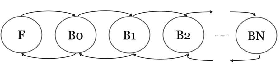
Figure 1.3: Transition diagram of cash desk queue

All events of a discrete event simulation system can be classified into the following categories:

• External events, independent of the behavior of the modeled system, are always present in the list of active events
• Internal events, which are a function of the system status, may or may not be present in the list of active events

The processes of arrival and departure of customers at a cash desk are completely characterized by probability distributions. It is essential to be able to evaluate, based on the data available, the probability distributions relating to the inter-arrival times of the tokens in the activities and the service of activities.

Another distinctive element of DES models is that the use of resources and activity times are specific to every single element of the system and are sampled using probability distributions. The rules governing the order in which the activities occur in the model are defined during the implementation phase of the model and are dependent on both how the workflow is structured and the characteristics of the individual entities.

The fundamental elements of a DES system are, therefore, the following:

• State Variables: Variables that describe the state of a system at any instant in time. In a DES model, the state variables take on discrete values, and the transitions from one state to another take place in discrete instants.
• Events: Any instantaneous occurrence that causes the value of at least one of the state variables to change.
• Activity: Temporal actions between two events, the duration of which is known a priori at the beginning of the execution of the activity.
• Entities and logical relationships: Entities are the tangible elements present in the real world, while logical relationships connect the different objects together, defining the general behavior of the model. Entities can be dynamic if they flow within the system or static entities. Entities can also be characterized by attributes that provide a data value assigned to the entity.
• Resources: Elements of the system that provide a service to entities.
• Simulation time: Keeps track of the logical relationships between entities in the time range to be simulated.

There are two ways to define the progress of the simulation time:

• Advancement of time to the next event: Time flows according to the events; it passes from the previous moment to the next one only according to the events associated with these moments
• Advancement of time in predetermined increments: Time flows regardless of the events; it passes from one instant before to the next regardless of the events associated with those instants

Finite-state machine (FSM)

To describe a DES in a simple way, we can adapt the FSM model. It is the first abstraction of a machine equipped with memory that executes algorithms. It introduces the fundamental concept of the state, which can be defined as a particular condition of the machine. As a result, the machine reacts with a certain output to a specific input. Since the output also depends on the state, FSM is an automaton intrinsically equipped with an internal memory that can therefore influence the answers given by the automaton. A system of this nature can be formally described with a quintuple of variables:

Here, we have the following variables:

• S is the finite set of possible states
• I is the possible set of input values
• O is the set of possible output values
• δ is the function that links inputs and the current state with the neighboring state
• is the initial state

The state contains the information necessary to calculate the system output, and in general, the inference of the sequence of inputs that brought the system to a certain state is not possible.

A system in which the output depends only on the current state is called Moore’s Machine. If the output depends on both the current state and the inputs, then it is called the Mealy Machine. In Moore’s machine, the outputs are connected to the current state of the system, whereas in Mealy’s machine, they are connected to the transitions from one state to another. The two automata are equivalent, that is, a system that can be created with one of the two models can always be created with the other model as well. In general, Mealy automata have fewer states than the corresponding Moore automata, even if they are more complicated to synthesize.

State transition table (STT)

The state of a state machine evolves in the presence of an event on the input or on the state itself. A sequential machine can be described by means of the state table. The column indices are the symbols of the input values, while the row indices are the state symbols that indicate, in the case of a Moore automaton, each possible current state, and for each combination of inputs, the next state reached by the automaton is indicated. Finally, a further column of the table expresses the relationship between the system status and the corresponding output.

State transition graph (STG)

The STG allows you to completely describe a finite state automaton through an oriented and labeled graph. It is a very useful graphic representation in the initial phases of the project, in which we pass from a formal description of the machine to its behavioral model. A node of the graph corresponds to each state. If a transition from state A to state B is possible in relation to input i, then on the graph, there will exist an arc oriented from the node corresponding to A to the node corresponding to B, labeled with i (Figure 1.2). In the case of Moore automata, in which the output is a function of the current state only, the indication of the output u corresponding to a state A is shown inside the node that identifies state A.

After exploring DES, we will now look at how to model dynamic systems.

In this section, we will analyze a real case of modeling a production process. In this way, we will learn how to deal with the elements of the system and how to translate the production instances into the elements of the model. A model is created to study the behavior of a system over time. It consists of a set of assumptions about the behavior of the system being expressed using mathematical-logical-symbolic relationships. These relationships are between the entities that make up the system. Recall that a model is used to simulate changes in the system and predict the effects of these changes on the real system. Simple models are resolved analytically using mathematical methods, while complex models are numerically simulated on the computer, where the model results are treated like data from a real system.

Managing workshop machinery

In this section, we will look at a simple example of how a discrete event simulation of a dynamic system is created. A discrete event system is a dynamic system whose states can assume logical or symbolic values, rather than numerical ones, and whose behavior is characterized by the occurrence of instantaneous events within an irregular timing sequence, not necessarily known a priori. The behavior of these systems is described in terms of states and events.

In a workshop, there are two machines that we will call A1 and A2. At the beginning of the day, five jobs need to be carried out: W1, W2, W3, W4, and W5. The following table shows the time (minutes) we need to work on the machines:

Table 1.1: Table showing work time on the machines

A zero indicates that a job does not require that machine. Jobs that require two machines must pass through A1 and then through A2. Suppose that we decide to carry out the jobs by assigning them to each machine so that when they become available, the first executable job is started first, in order from 1 to 5. If at the same time, more jobs can be executed on the same machine, we will execute the one with a minor index first.

The purpose of modeling is to determine the minimum time needed to complete all the work. The events in which state changes can occur in the system are as follows:

• A job becomes available for a machine
• A machine starts a job
• A machine ends a job

Based on these rules and the evaluation times indicated in the previous table, we can insert the sequence of the jobs, along with the events scheduled according to the execution times, into a table:

Table 1.2: Table of job sequences

This table shows the times of the events in sequence, indicating the start and end of the work associated with the two machines available in the workshop. At the end of each job, a new job is sent to each machine according to the rules set previously. In this way, the deadlines for the work and the subsequent start of another job are clearly indicated. This is just as easy as it is to identify the time interval in which each machine is used and when it becomes available again. The table solution we have proposed represents a simple and immediate way of simulating a simple dynamic discrete system.

The example we just discussed is a typical case of a dynamic system in which time proceeds in steps in a discrete way. However, many dynamic systems are best described by assuming that time passes continuously. In the next section, we will analyze the case of a continuous dynamic system.

Simple harmonic oscillator

Consider a mass m, resting on a horizontal plane, without friction, and attached to a wall by an ideal spring, of elastic constant k. Suppose that when the horizontal coordinate x is zero, the spring is at rest. The following diagram shows the scheme of a simple harmonic oscillator:

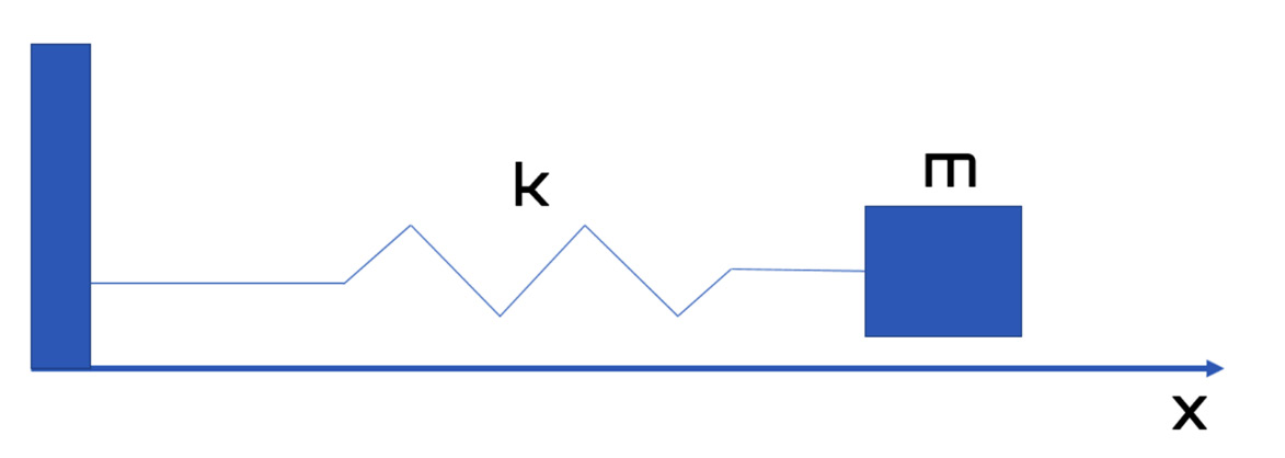
Figure 1.4: The scheme of a harmonic oscillator

If the block of mass m is moved to the right with respect to its equilibrium position (x> 0), the spring being elongated pulls it to the left. Conversely, if the block is placed to the left of its equilibrium position (x < 0), then the spring is compressed and pushes the block to the right. In both cases, we can express the component along the x axis of the force due to the spring according to the following formula:

Here, we have the following:

• is the force
• is the elastic constant
• is the horizontal coordinate that indicates the position of the mass m

From the second law of dynamics, we can derive the component of acceleration along x as follows:

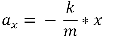
Here, we have the following:

• is the acceleration
• is the elastic constant
• is the mass of the block
• is the horizontal coordinate that indicates the position of the mass m

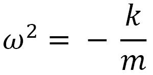
If we indicate with the rate of change of the speed and with the speed, we can obtain the evolution equations of the dynamic system, as follows:

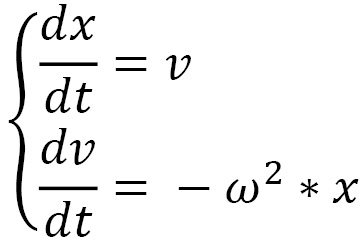
Here, we have the following:

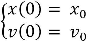
For these equations, we must associate the initial conditions of the system, which we can write in the following way:

The solutions to the previous differential equations are as follows:

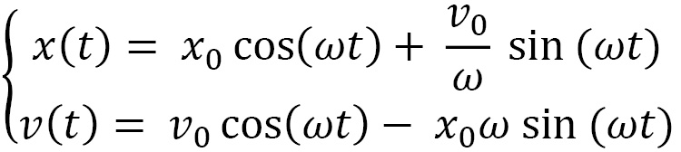
In this way, we obtained the mathematical model of the analyzed system. To study the evolution of the oscillation phenomenon of the mass block m over time, it is enough to vary the time and calculate the position of the mass at that instant and its speed.

In decision-making processes characterized by high levels of complexity, the use of analytical models is not possible. In these cases, it is necessary to resort to models that differ from those of an analytical type for the use of the calculator as a tool not only for calculation, such as in mathematical programming models but also for representing the elements that make up reality while studying the relationships between them.

The predator-prey model

In the field of simulations, simulating the functionality of production and logistic processes is considerably important. These systems are, in fact, characterized by high complexity, numerous interrelationships between the different processes that pass through them, segment failures, unavailability, and the stochasticity of the system parameters.

To understand how complex the analytical modeling of some phenomena is, let’s analyze a universally widespread biological model. This is the predator-prey model, which was developed independently by the Italian researcher Vito Volterra and the American biophysicist Alfred Lotka.

On an island, there are two populations of animals: prey and predators. The vegetation of the island provides the prey with nourishment in quantities that we can consider as unlimited, while the prey is the only food available for predators. We can consider the birth rate of the prey constant over time; this means that in the absence of predators, the prey would grow by exponential law. Their mortality rate, on the other hand, depends on the probability they have of falling prey to a predator and, therefore, on the number of predators present per unit area.

As for predators, the mortality rate is constant, while their growth rate depends on the availability of food and, therefore, on the number of prey per unit area present on the island. We want to study the trend of the size of the two populations over time, starting from a known initial situation (number of prey and predators).

To carry out a simulation of this biological system, we can model it by means of the following system of finite difference equations, where x(t) and y(t) are the numbers of prey and predators at time t, respectively:

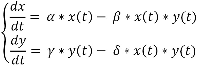
Here, we have the following:

• α, β, γ, δ are positive real parameters related to the interaction of the two species
• is the instantaneous growth rate of the prey
• is the instantaneous growth rate of the predators

The following hypotheses are underlined in this model:

• In the absence of predators, the number of prey increases according to an exponential law, that is, at a constant rate
• Similarly, in the absence of prey, the number of predators decreases at a constant rate

This is a deterministic and continuous simulation model. In fact, the state of the system, represented by the size of the two populations in each instance of time, is univocally determined by the initial state and the parameters of the model. Furthermore, at least in principle, the variables – that is, the size of the populations – vary continuously over time.

The differential system is in normal form and can be solved with respect to the derivatives of maximum order but cannot be separated into variables. It is not possible to solve this in an analytical form, but with numerical methods, it is solved immediately (Runge-Kutta method). The solution obviously depends on the values of the four constants and the initial values.

After analyzing how to model dynamic systems, let’s see step by step how to perform a simulation of a real system.

To perform a correct simulation, the simulation software must be properly structured. The program structure must consist of three software levels:

• The simulation executive software controls the execution of the model program. It sequences operations and manages modularity problems by separating generic control from model details. Two techniques are possible: the synchronous execution technique and the event-scanning technique.
• The model program implements the model of the system to be simulated and is executed by the simulator.
• The routine tools generate random numbers by deriving them from typical probability distributions to obtain statistics and to manage problems related to modularity by separating generic functions from those specific to the model.

The main cycle of a simulation generally consists of three phases:

• Start phase: The termination condition is initialized to false; the status variables are initialized, the clock is set to the simulation start time (usually zero), and the initial events are placed in the event list.
• Loop phase: The cycle continues until the termination condition occurs. At each step, the clock is set equal to the start time of the first event in the queue, the event is simulated and removed from the queue, and finally, the statistics are updated.
• End phase: The simulation ends by generating a report with the statistics of the simulated system.

The simulation can be applied to all systems that can be modeled, respecting the characteristics mentioned in the previous paragraphs. This approach is particularly suitable for diagnosing problems related to complex processes. Understand where the system bottlenecks are. These areas are critical as they significantly decrease system performance and are usually associated with slower components. The only way to significantly improve the performance of a process is to improve it precisely in these critical areas, which, unfortunately, in many processes, are clouded by excess inventory, overproduction, diversity of processes, different sequencing, and stratification.

Therefore, by modeling these processes accurately and inserting them into a simulator, it is possible to obtain a more detailed view of the entire system, find the bottlenecks, and use performance indicators to analyze the system and improve its performance.

A simulation is a numerical model that mimics the operations of a real existing system, such as the daily operations of a bank, the process of a factory assembly line, and the assignment of personnel in a hospital or call center. For this reason, it must consider all the resources and constraints related to the system and their interactions over time. It must also coincide as much as possible with reality and therefore consider that events can have variable completion times, and this is done by introducing pseudorandom generators. In this way, the simulation is much closer to the real situation, and therefore through it, it is possible to predict the behavior of the system in the face of changes in the input data or its structure, just as if the simulation were real. Therefore, with this type of simulation, you can test your ideas much faster and at a much lower cost than real simulation.

Generally, any real system that is expressible through a flow of processes with events can be simulated. The processes that can be most beneficial are those with more changes over time and with a high level of randomness. A good example is a vehicle filling station: you cannot predict exactly when the next customer will arrive, nor the type and quantity of fuel they will require.

Consequently, the simulation, where applicable, should be preferred to the real simulation since a gain in terms of cost, time, and repeatability of the simulation is obtained. Just think of the cost associated with each real simulation, not only as regards the expense of hiring new employees or purchasing new components, but also the consequences that these decisions can have on the real system, which can lead to positive but also negative results. On the other hand, this is avoidable in numerical simulation in which the system has no connections with the real system, and therefore the test does not cause economic consequences.

Furthermore, it is more difficult to simulate the same real system twice with the same conditions, while in numerical simulation, you can test a system with the same conditions by modifying only the input. This gives greater certainty that one idea is better than another. Finally, as mentioned before, the time needed to carry out a numerical simulation is much shorter than that of a real simulation, especially if the simulated system takes a very long time. For example, if we want to analyze the throughput of customers in a month, the real simulation must pass at least 1 month, and the numerical one just a few seconds.

In this chapter, we learned what is meant by simulation modeling. We understood the difference between modeling and simulation, and we discovered the strengths of simulation models, such as defects. To understand these concepts, we clarified the meaning of the terms that appear most frequently when dealing with these topics.

We then analyzed the different types of models: static versus dynamic, deterministic versus stochastic, and continuous versus discrete. We then explored the workflow connected to a numerical simulation process and highlighted the crucial steps. Furthermore, we analyzed in detail the discrete event systems that simulate a dynamic system whose states can take on logical or symbolic, rather than numerical, values. Finally, we studied some practical modeling cases to understand how to elaborate on a model starting from the initial considerations.

In the next chapter, we will learn how to approach a stochastic process and understand the random number simulation concepts. Then, we will explore the differences between pseudo and non-uniform random numbers, as well as the methods we can use for random distribution evaluation